Planning by imagination, on a toy world
A concrete take on the world-models program: train a small world model on a 2D navigation task, plan with the dumbest possible MPC, and check what actually does the work.
I wanted to see whether the world-models pitch — an agent imagines actions in latent space and picks the best one — holds together on a problem small enough to debug. So I built one: a 2D dot world with a wall, a small world model (an encoder that maps frames to latents, plus a predictor that rolls those latents forward under an action — the JEPA recipe), and a planner that scores imagined rollouts.
The planner is shooting MPC — Model Predictive Control. At each real step: sample a bunch of random action sequences, imagine each one \(H\) steps forward through the predictor, score them, take the first action of the best sequence, then replan from the new real state. \(H\) is the horizon — how far ahead the agent imagines before committing to one real action. “Shooting” just means we sample the sequences instead of optimizing them.
Three claims up front:
- Encoder — easy. Anti-collapse regularizers produce a latent that recovers the world’s geometry, including a wall that’s invisible in pixels.
- Predictor — silent overfit. Training past the right epoch quietly degrades planning while every standard proxy keeps improving. One held-out signal catches it without ever running the planner.
- Planner — the cost function dominates. Swapping endpoint cost for closest-approach cost lifts even the oracle planner from half the episodes to all of them at \(H = 20\). More impact than any encoder or predictor choice.
Scope: one narrow setting — 2D, two rooms, MPC navigation. Several claims lean on an analytic geodesic that exists because the world is small enough to write down.
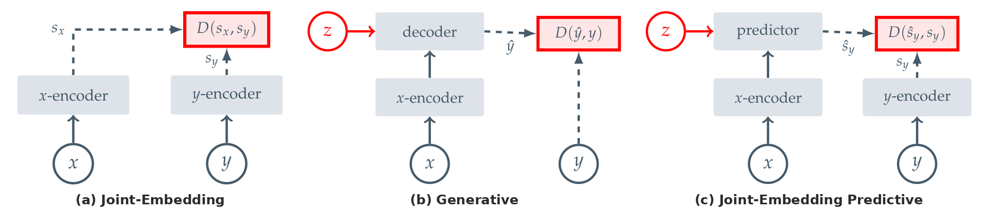
Where JEPA sits among self-supervised architectures. (a) Joint-Embedding encodes both views and pulls compatible embeddings together — no prediction. (b) Generative decodes a reconstruction \(\hat{y}\) back in input (pixel) space from \(x\) and a latent \(z\). (c) Joint-Embedding Predictive (JEPA) predicts the embedding of \(y\) from \(x\) in latent space via a predictor conditioned on \(z\) — it never decodes to pixels. That encoder + predictor pair is what this post builds on. Figure from Assran et al., I-JEPA (2023).
The toy world
The world is a 2D \(64 \times 64\) grid. A point \((x, y)\) renders as a slightly diffuse grayscale spot. A vertical wall at \(x = 1/2\) has a gap at \(y \in [0.4, 0.6]\). Goal: navigate from one room to the other.
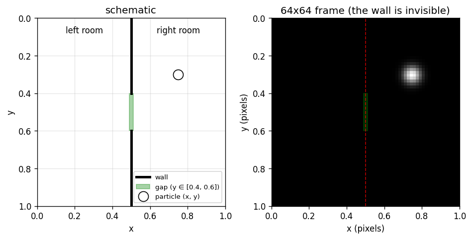
Figure 1: The left panel’s red dashed wall and green gap are reader-only — the right panel is what the encoder sees. The wall is invisible in pixels.
I trained the encoder + predictor on transitions \((s_t, a_t, s_{t+1})\) with latent-space MSE:
# Core JEPA step — single-step latent MSE plus a collapse regularizer
z_t      = encoder(obs_t)
z_next   = encoder(obs_next)
z_hat    = predictor(z_t, action)
loss_mse = F.mse_loss(z_hat, z_next.detach())
loss     = loss_mse + collapse_reg(z_t, z_next)
The encoder never sees pixels of the wall. Whether it learns the wall depends on which transitions the predictor sees fail.
Three diagnostics I use throughout:
- Probe \(R^2\) — linear readout from \(z\) to \((x, y)\). Saturates near 1 for any non-collapsed encoder; useful as a sanity check, useless for ranking.
- Intrinsic dim — 2-nearest-neighbor estimator of the latent manifold’s dimension; should land near 2 for this world.
- Geodesic correlation \(r(\delta z, \delta s_{\text{geodesic}})\) — Pearson correlation between latent distance \(\lVert z_a - z_b \rVert\) and the analytic wall-aware shortest-path distance. Especially on cross-room pairs. This is the one that does the work later.
Two encoders show up most:
- The primary — a SIGReg encoder with a residual predictor; highest scorer on the canonical MPC suite.
- The thin-predictor variant — same regularizer, but a thin single-layer predictor that emits the next latent directly rather than a delta from the current one. Same canonical score, different geometry — and it behaves differently when things get hard.
Encoder: a usable latent is easy to get
Once you defeat the trivial collapse, getting a JEPA encoder that internalizes this world is not hard, and not very sensitive to which regularizer you pick.
JEPA’s loss is satisfied by a constant encoder — everything maps to one point, predictor learns the constant, latent is useless. Anti-collapse regularizers fix this. The ones that worked:
- VICReg — variance hinge + off-diagonal covariance penalty. Standard JEPA recipe.
- SIGReg (from LeJEPA) — projects the latent onto random 1D slices, pushes each slice toward unit Gaussian. A goodness-of-fit penalty instead of a moment penalty.
The ones that didn’t:
- Bisimulation-style oracle distillation — scale-collapsed in practice.
- Sliced Wasserstein to N(0, I) — prevented collapse but stayed wall-blind.
- SimSiam-style asymmetry — found degenerate shortcuts.
Naïve collapse, VICReg fix
Without regularization, validation loss drops to zero but the linear probe stays at chance. VICReg’s variance hinge prevents the degenerate solution.
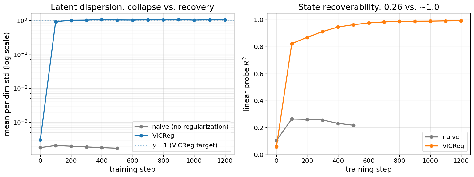
Figure 2: Naïve std collapses 5 orders of magnitude; VICReg holds at \(\gamma=1\) and probe \(R^2\) saturates near 1.
Where the latent ends up
Once collapse is prevented, the first two PCs of the latent are essentially the world coordinates — and the room topology appears in PCA space without ever being told to:
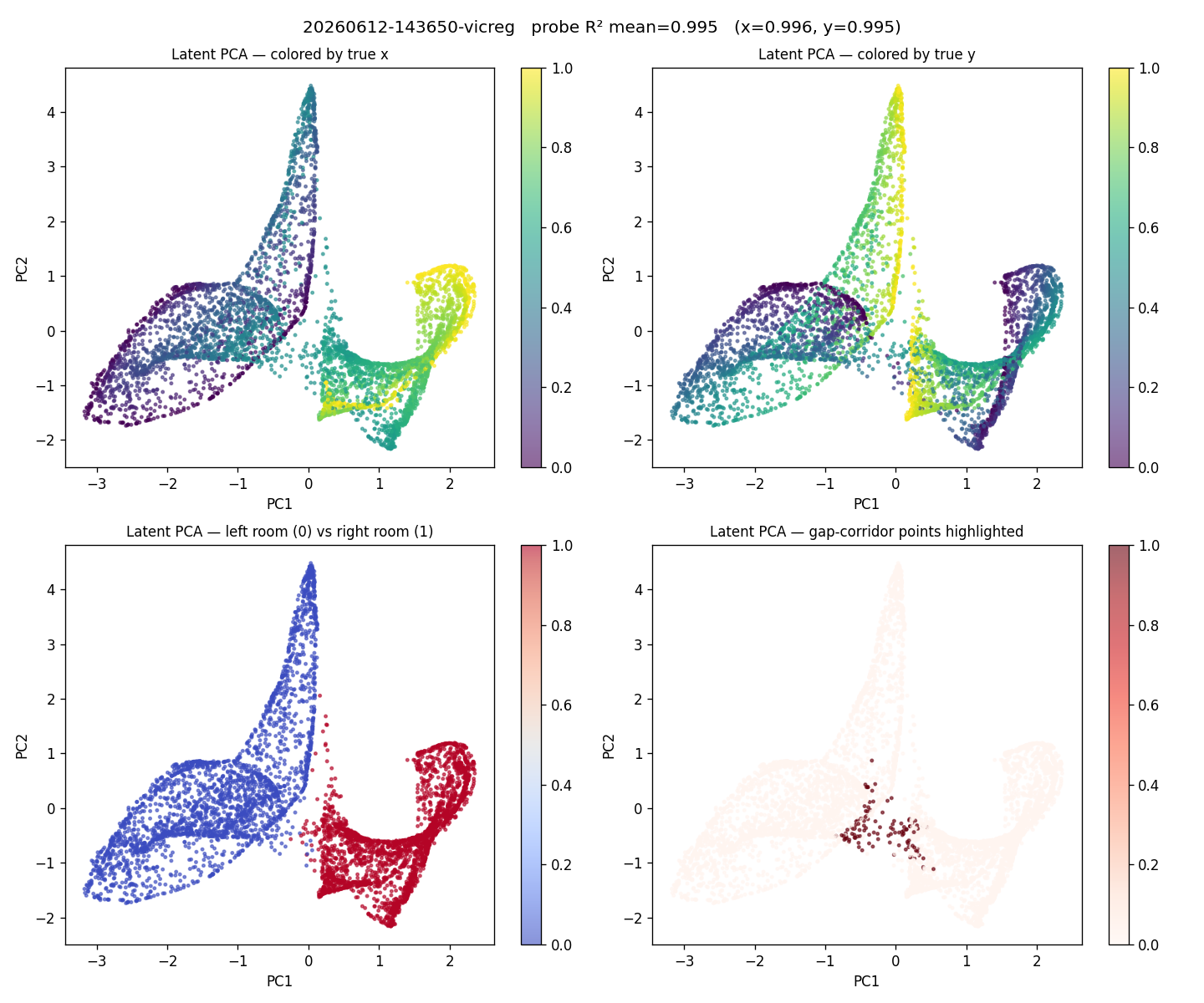
Figure 3: PC1/PC2 colored by ground-truth \(x\), \(y\) (top) and by room membership (bottom). The encoder discovered the wall from blocked transitions alone.
That’s the sentence I find most encouraging for the broader program, and the one that took me longest to fully believe.
Probe \(R^2\) is saturated; use geodesic-r instead
Probe \(R^2 \approx 1.0\) for every non-collapsed encoder, so it can’t rank them. Scattering latent distance against the wall-aware geodesic does:
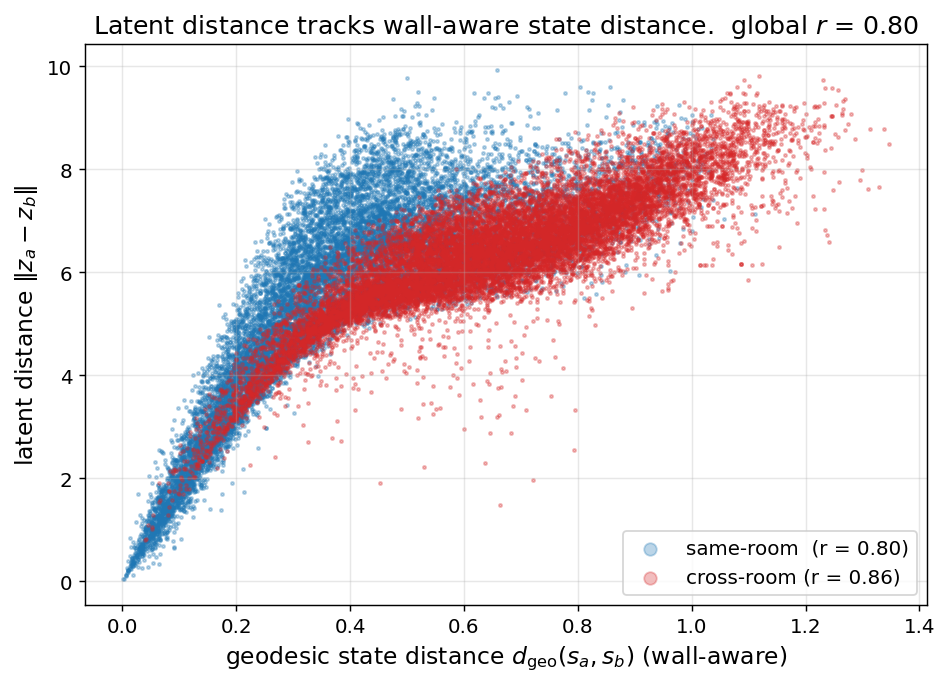
Figure 4: Latent distance vs wall-aware geodesic. Cross-room pairs (red) track the geodesic, not the Euclidean distance through the wall.
Across non-collapsed encoders, cross-room \(r\) runs from about 0.74 to 0.89 — enough to rank them, where probe \(R^2\) can’t. The wall-blind SW encoder sits at 0.53, its wall essentially invisible in the latent.
Predictor: a silent overfit, with an MPC-free signal
Once the encoder is in place, the predictor is the easier of the two bottlenecks — but its failure mode is silent. Training longer keeps lowering validation loss and raising prediction SNR while downstream MPC quietly degrades.
(SNR here = ratio of per-step latent motion to per-step prediction error. Higher is better.)
Freezing the encoder isolates the predictor
The cleanest test: freeze the encoder at a known-good checkpoint and train only the predictor.
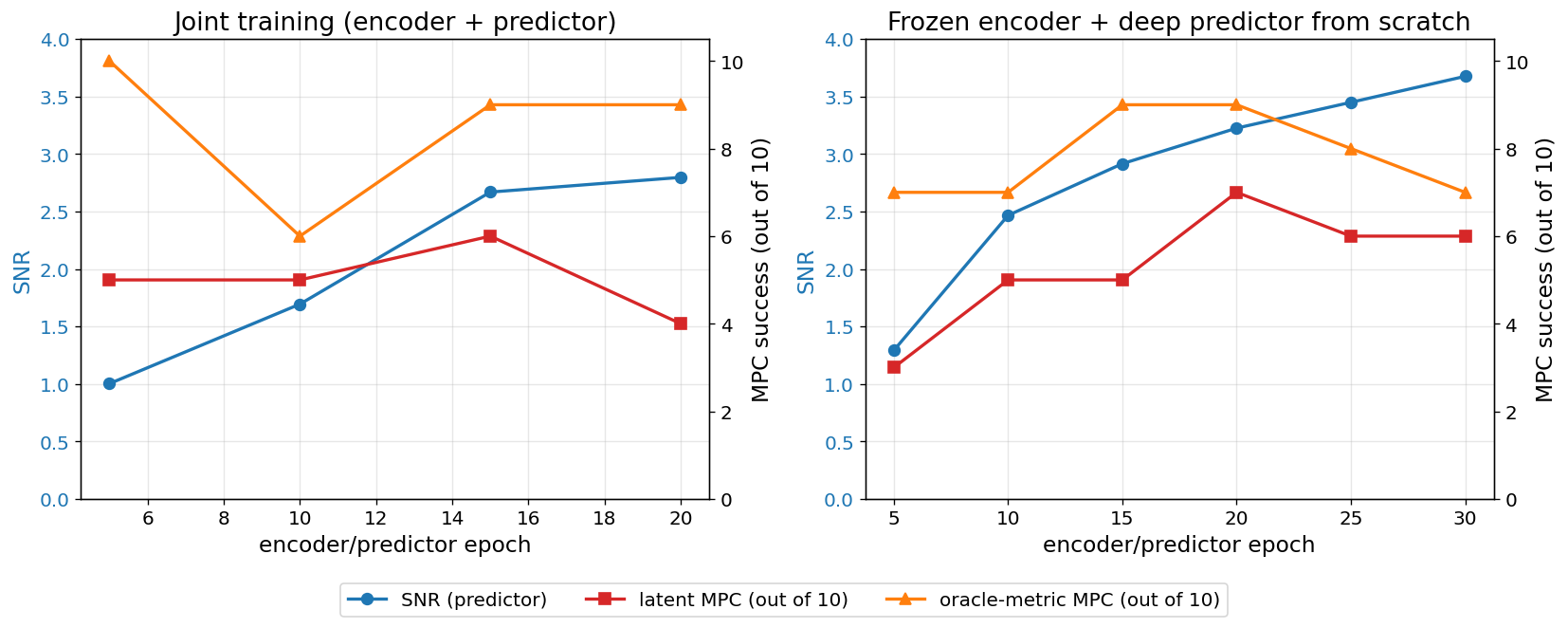
Figure 5: Joint training (left) vs frozen-encoder + deep predictor (right). In both panels SNR climbs steadily; in both, MPC peaks mid-training and drifts down — the late-training gap between “predictor still improving” and “planning getting worse” is the silent overfit.
SNR triples — the predictor was underfit in joint training. But oracle-metric MPC peaks mid-training and drifts back down, even as SNR keeps climbing and validation MSE keeps falling. Late in training the predictor is still lowering its per-frame MSE, but my read is that it’s fitting the held-out frames’ specifics rather than the shape of motion — and the frames it nails aren’t necessarily the ones MPC ends up rolling out.
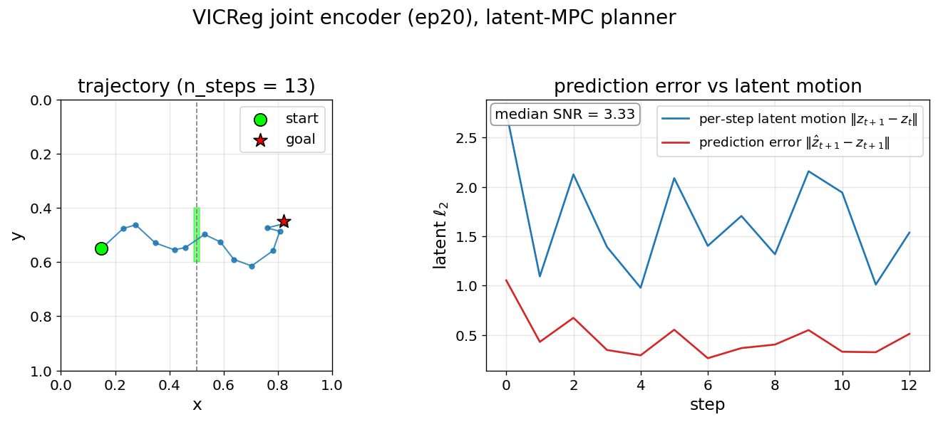
Figure 6: One MPC episode. Per-step prediction error sits below per-step motion but in the same order of magnitude — that compounding is what bounds rollout horizon.
The MPC-free overfit signal
The interesting bit. Across joint training, probe \(R^2\) stays pinned near 1 and SNR climbs monotonically — both happy while MPC is dying. But geodesic correlation on a held-out batch drops on the same epochs MPC declines. Same pattern on the historical baseline.
That’s a candidate stopping rule that doesn’t require running the planner: compute \(r(\delta z, \delta s)\) on a held-out batch each epoch, stop when it stops climbing.
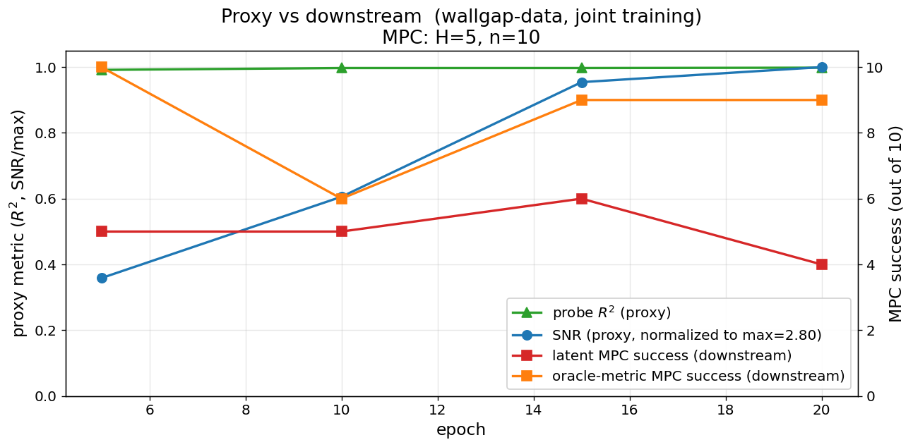
Figure 7: Across joint training, the standard proxies (probe \(R^2\), SNR) keep improving while both MPC scores peak and fall. Geodesic-r — not shown — drops over the same window, so it’s the one proxy that would tell you to stop.
The honest caveat: this geodesic distance exists because I can write down the shortest-path-through-the-gap analytically. In a world where I can’t, this diagnostic doesn’t transfer as-is — that’s a Part 2 question.
MPC: the cost function is the bottleneck
The biggest single lever in this whole pipeline isn’t the encoder or the predictor. It’s how you score a rollout — at least once there’s a rollout to score; at \(H = 1\), with no rollout at all, that flips, as the \(H = 1\) section below shows.
What shooting MPC is doing
Spelling out the recipe with the actual symbols. Given start state \(s_0\) and goal \((x^*, y^*)\):
- Encode the goal once: \(z^* = \mathrm{Enc}(\mathrm{Render}(x^*, y^*))\).
- At step \(t\), encode the current observation: \(z_t = \mathrm{Enc}(s_t)\).
- Sample \(N\) action sequences of length \(H\). I used \(N = 1000\), \(H \in \{5, 20\}\), uniform i.i.d. with \(\lVert a \rVert \le 0.08\).
- Roll out each sequence in latent space through the predictor.
- Score each trajectory. ← The dial.
- Take the first action of the best sequence; apply it to the real world.
- Repeat.
The cost runs on the predicted latent trajectory \(\{\hat z_t\}\) against \(z^*\). Using ground-truth \((x, y)\) would be cheating — the point is to learn whether the latent stack stands in for the oracle.
# One real step of shooting MPC
z_t      = encoder(obs_t)
actions  = sample_actions(N, H)                          # (N, H, 2)
z_traj   = rollout(predictor, z_t, actions)              # (N, H, d)
costs    = score(z_traj, z_goal)                         # (N,)  endpoint or min-traj
first_action = actions[costs.argmin(), 0]
Two cost functions
Two natural ways to summarize a rollout against the encoded goal \(z^\ast\):
Endpoint cost — score by the final predicted state: \(J_\text{endpoint}\big(\hat{z}_{1:H}\big) = \lVert \hat{z}_H - z^\ast \rVert.\)
Min-trajectory cost — score by the closest approach across all timesteps: \(J_\text{min-traj}\big(\hat{z}_{1:H}\big) = \min_{t \in [1, H]} \lVert \hat{z}_t - z^\ast \rVert.\)
Endpoint is the textbook default — it’s what “terminal cost” means in classical MPC, and what most learned-MPC papers use without comment.
Why use a long horizon at all? A short rollout can’t see trajectories that require setup: if the goal is across the wall, a one-step plan from far away can’t anticipate threading the gap. Longer \(H\) buys visibility into payoffs several steps away. But once a candidate reaches the goal at step 8, why insist on scoring it by step 20? Min-trajectory lets the planner use the full horizon to find good candidates while committing to the part of each candidate that actually solves the task.
The cost rule decides everything
Same \(N = 1000\), same shooting, same wall, same predictor; only the rule for scoring rollouts changes. Below: solve rate on a 30-episode canonical suite.
| model | metric | \(H\) | endpoint | min-trajectory |
|---|---|---|---|---|
| oracle | Euclidean | 5 | 30/30 | 30/30 |
| oracle | Euclidean | 20 | 15/30 | 30/30 |
| oracle | geodesic | 20 | 14/30 | 29/30 |
| learned (primary) | latent | 5 | 28/30 | 28/30 |
| learned (primary) | latent | 20 | 8/30 | 28/30 |
| learned (thin-predictor) | latent | 5 | 27/30 | 30/30 |
| learned (thin-predictor) | latent | 20 | 27/30 | 29/30 |
The cleanest fact in the post is the oracle + Euclidean row at \(H = 20\): half the episodes under endpoint, all of them under min-trajectory. No encoder, no predictor, no metric noise — just a different scalar summary of the rollout.
So the “long-horizon shooting MPC is hard” reading I’d been working with isn’t really about long horizons at all. It’s about overshoot. A random-walk rollout that hits the goal at step 8 doesn’t stop — by step 20 it’s wandered off again, and endpoint cost throws it out. The planner ends up committing to the first action of some other sequence whose end happens to land near the goal — almost certainly a contrived trajectory. Min-trajectory fixes this directly: it rewards the rollout that passed through the goal at step 8, regardless of where it ended up later.
Under min-trajectory, the thin-predictor variant is saturated at both horizons on the canonical suite. The encoders that internalized the wall all cluster near the oracle ceiling; the gap between them shows up at \(H = 5\) and closes at \(H = 20\) — once the rollout is long enough, almost any candidate sequence brushes near the goal at some step, and min-trajectory rewards that. So \(H = 5\) is where regularizer-specifics discriminate; \(H = 20\) is a saturation check.
Min-trajectory unlocks encoders that already had usable geometry; it doesn’t save the ones that didn’t. That’s roughly the right behavior: a cost function should expose the encoder’s geometry, not paper over its failures.
\(H = 1\) on hard cross-wall: metric vs rollout are partial substitutes
Headline claim: metric quality and rollout depth substitute for the same information — wall geometry. A true geodesic metric makes per-step greedy planning sufficient. If the metric is missing the wall, longer rollouts can recover by putting wall-threading trajectories into the candidate set. You can have one or the other.
To probe this I shrunk the horizon to \(H = 1\): no rollout at all, just per-step greedy in latent space. If the metric is wall-aware pointwise, that should suffice.
I built a 30-episode hard cross-wall suite: start and goal both close to the wall on opposite sides. Half the episodes are far-from-gap — both points sit near the top or bottom edge, far from the gap at \(y \in [0.4, 0.6]\). These have a specific property: any solving trajectory must be non-monotonic in \(y\) — the agent has to move away from the goal-\(y\) to reach the gap, then back. The other half are spread — long \(y\) traversal plus a gap thread.
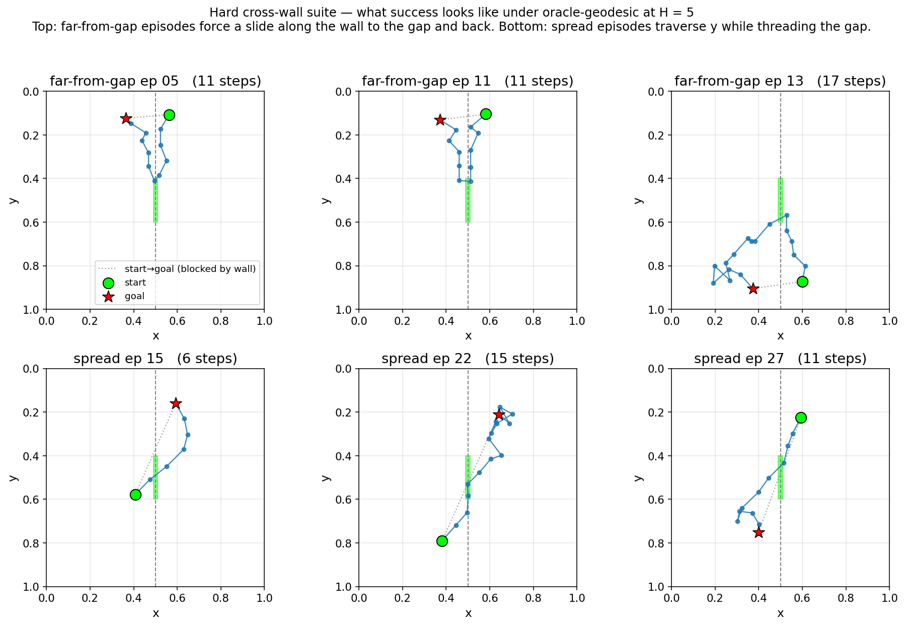
Figure 8: Six hard episodes under oracle-geodesic at \(H = 5\). Top — far-from-gap: a large detour from goal-\(y\) to thread the gap. Bottom — spread: long diagonals routed through the gap.
Oracle reference. With a perfect metric (oracle-geodesic) and no rollout at all, the planner solves every episode. With a straight-line metric (oracle-Euclidean), it solves only the easy half and fails every far-from-gap episode — the gradient pulls it through the wall. But give that same straight-line metric \(H = 20\) and it recovers to a perfect score: the rollout puts gap-threading sequences in the candidate set, and min-trajectory ranks them correctly.
The learned encoders all fall below the oracle ceiling at \(H = 1\), harshly:
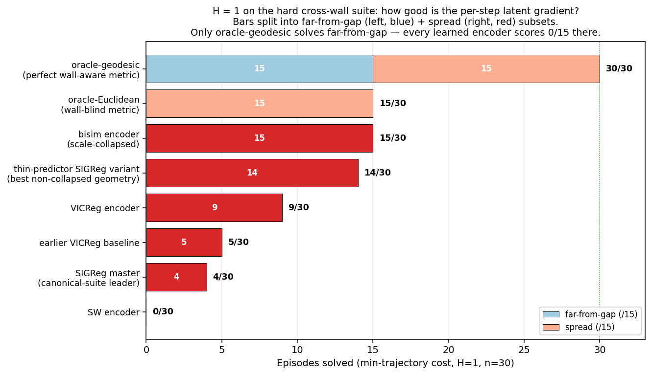
Figure 9: Only oracle-geodesic solves far-from-gap at \(H = 1\). Every learned encoder, and oracle-Euclidean, fails every far-from-gap episode — their solves all come from the easier spread subset.
The thin-predictor variant is the best learned encoder at \(H = 1\) — but every one of its wins is a spread episode. Give the primary \(H = 20\) and it jumps from near-zero to 27 of 30 (90%), including most of the far-from-gap episodes. The rollout patches what the encoder didn’t learn:
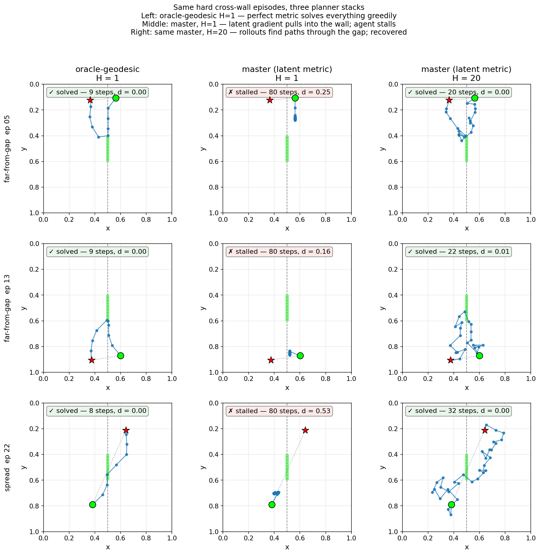
Figure 10: Three hard episodes, three planner stacks. Left — oracle-geodesic \(H = 1\): solved quickly. Middle — primary \(H = 1\): stalls; the latent gradient pulls toward the goal *through the wall. Right — same encoder \(H = 20\): rollouts find gap-threading sequences. Rollout-mediated vs metric-mediated, side by side.*
Two things worth pulling out:
- The \(H = 1\) ranking diverges from the canonical-suite ranking. The canonical #1 is near-zero at \(H = 1\); the best learned encoder at \(H = 1\) still fails every far-from-gap episode.
- Most learned-pipeline performance is rollout-mediated. With horizon, learned encoders cluster near the oracle ceiling; the horizon is compensating for what the encoder didn’t learn.
So MPC at \(H = 1\) on a non-monotonic-required suite is the cleanest single number for “did this encoder learn the world’s geometry pointwise.” By that measure, no encoder here makes it. The earlier “encoder is easy to get” claim was scoped to good-enough-for-\(H = 5\); the pointwise regime is genuinely open.
Takeaways
Three things I think survive this experiment:
-
Self-supervised representations recover world geometry from dynamics alone. The wall is invisible in pixels, yet multiple encoders learn it from “which transitions never happen.” This is the part of LeCun’s program I find most concretely supported here.
-
Planning by imagination works. With the right cost, learned-encoder + learned-predictor MPC lands within one episode of the oracle ceiling on the canonical suite. Even on the hard cross-wall suite, where the encoder fails per-step, the rollout patches what the encoder didn’t learn — 27 of 30 at \(H = 20\).
-
Interfaces matter more than components. I spent the most time chasing the wrong bottleneck (the encoder’s latent metric) and not enough on the right one (the cost function consuming that metric). JEPA stacks should probably ship with a cost-function ablation as a default debugging step.
Three things this doesn’t show:
- Whether geodesic-r as a stopping signal generalizes. It works here because I have an analytic oracle. Open whether learned surrogates (graph distance on a k-NN over latents, learned bisimulation metric, action-cost distance) carry the same signal.
- Whether the cost-rule lesson scales. Min-trajectory is the right answer for “navigate to a point” — closest approach is what success means. For other tasks the right summary is different (return, value function, time-to-event). The structural point — cost is an editorial choice masquerading as a scoring detail — should transfer; the recipe shouldn’t.
- Whether 16 latent dims for a 2D world is teaching me anything about real worlds. Several diagnostics here are dominated by the fact that the true manifold is very low-dimensional.
What’s next
Two threads, each genuinely open:
- Oracle-free overfit signals. Build candidate replacements for geodesic-r: graph distance on a learned k-NN over latents, action-cost distance, learned bisimulation metric. Test whether any of them track downstream MPC the way the analytic geodesic does.
- Encoder shape, not loss. Across working regularizers, regularizer choice contributes a handful of episodes at \(H = 5\) and effectively nothing at \(H = 20\) under min-trajectory. The bigger lever might be encoder shape — latent dim, predictor depth, residual vs absolute mode, freeze vs joint training.
If you’ve worked with world models on tasks involving navigation, long horizons, or planning by imagination — what showed up that this toy world is missing? Which claims here do you expect to break first on a less toy problem? Find me on Twitter.
References
- LeCun’s World Models program — A Path Towards Autonomous Machine Intelligence (2022), PDF.
- VICReg — Bardes, Ponce & LeCun, arXiv:2105.04906.
- LeJEPA / SIGReg — Balestriero & LeCun, arXiv:2511.08544.
- MPC (classical) — Camacho & Bordons, Model Predictive Control (Springer, 2nd ed.).
- PlaNet — Hafner et al., arXiv:1811.04551. Closest published-system analogue: latent world model + planning in latent space.
- Dreamer — Hafner et al., arXiv:1912.01603. Successor to PlaNet; trains a policy on imagined rollouts.